Algorithms

They are following different formulas to compute Hamming windows

• In R, it is

(25/46) – (21/46) * cos(2 * pi * (0:n)/N)

which can be viewed when typing hamming

> hamming
function (n, method = c("symmetric", "periodic")) 
{
    if (!isPosscal(n) || !isWhole(n) || n <= 0)
        stop("n must be an integer strictly positive")
    method <- match.arg(method)
    if (method == "periodic") {
        N <- n
    }
    else if (method == "symmetric") {
        N <- n - 1
    }
    else {
        stop("method must be either 'periodic' or 'symmetric'")
    }
    if (n == 1) {
        w <- 1
    }
    else {
        n <- n - 1
        w <- (25/46) - (21/46) * cos(2 * pi * (0:n)/N)
    }
    w
}

• In MATLAB, the algorithm is (see https://se.mathworks.com/help/signal/ref/hamming.html)

and there are some precision difference for two coefficients

> 25/46
[1] 0.5434783
> 21/46
[1] 0.4565217

Analysis

Two reasons that make the differences

1. in gsignals::hamming, if you choose symmetric by default, you will have N <- n-1 and n <- n-1, that means the equivalent to Matlab’s hamming should be hamming(76+1)
2. the approximations 0.54 and 0.46 in Matlab contribute to the deviation from R’s version.

Tests with Handmade Implementations

We can implement hamming functions according to formulas from MATLAB and R, respectively, e.g.,

hamMatalb <- function(n) 0.54 - 0.46 * cos(2 * pi * (0:n) / n)
hamR <- function(n) 25 / 46 - 21 / 46 * cos(2 * pi * (0:n) / n)

and then run

> hamMatalb(75) # the same as obtained by hamming(76) in MATLAB
 [1] 0.08000000 0.08161328 0.08644182 0.09445175 0.10558687 0.11976909
 [7] 0.13689893 0.15685623 0.17950101 0.20467443 0.23219992 0.26188441
[13] 0.29351967 0.32688382 0.36174283 0.39785218 0.43495860 0.47280181
[19] 0.51111636 0.54963351 0.58808309 0.62619540 0.66370312 0.70034314
[25] 0.73585847 0.77000000 0.80252824 0.83321504 0.86184514 0.88821773
[31] 0.91214782 0.93346756 0.95202741 0.96769718 0.98036697 0.98994790
[37] 0.99637276 0.99959650 0.99959650 0.99637276 0.98994790 0.98036697
[43] 0.96769718 0.95202741 0.93346756 0.91214782 0.88821773 0.86184514
[49] 0.83321504 0.80252824 0.77000000 0.73585847 0.70034314 0.66370312
[55] 0.62619540 0.58808309 0.54963351 0.51111636 0.47280181 0.43495860
[61] 0.39785218 0.36174283 0.32688382 0.29351967 0.26188441 0.23219992
[67] 0.20467443 0.17950101 0.15685623 0.13689893 0.11976909 0.10558687
[73] 0.09445175 0.08644182 0.08161328 0.08000000

> hamR(75) # the same as obtained by gsignal::hamming(76) in R
 [1] 0.08695652 0.08855761 0.09334964 0.10129899 0.11234992 0.12642490
 [7] 0.14342521 0.16323161 0.18570516 0.21068824 0.23800559 0.26746562
[13] 0.29886168 0.33197355 0.36656897 0.40240529 0.43923112 0.47678818
[19] 0.51481302 0.55303893 0.59119778 0.62902190 0.66624601 0.70260898
[25] 0.73785576 0.77173913 0.80402141 0.83447617 0.86288979 0.88906296
[31] 0.91281211 0.93397064 0.95239015 0.96794144 0.98051542 0.99002390
[37] 0.99640019 0.99959955 0.99959955 0.99640019 0.99002390 0.98051542
[43] 0.96794144 0.95239015 0.93397064 0.91281211 0.88906296 0.86288979
[49] 0.83447617 0.80402141 0.77173913 0.73785576 0.70260898 0.66624601
[55] 0.62902190 0.59119778 0.55303893 0.51481302 0.47678818 0.43923112
[61] 0.40240529 0.36656897 0.33197355 0.29886168 0.26746562 0.23800559
[67] 0.21068824 0.18570516 0.16323161 0.14342521 0.12642490 0.11234992
[73] 0.10129899 0.09334964 0.08855761 0.08695652

and we can check the lengths of resulting windows

> length(hamMatalb(75))
[1] 76

> length(hamR(75))
[1] 76

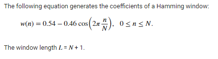
Spectral Performance

Given n <- 75, we can take a look at the difference in the frequency domain, using freqz. We can see that the difference mainly lies in the stopband but still quite minor, which doesn’t affect the filtering performance too much.

• freqz(hamR(n))

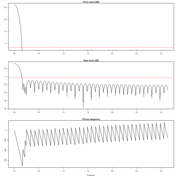
• freqz(hamMatlab(n))